Rendering Option Settings

Contents

• 105.1 Introduction
• 105.2 PK_GEOM_render option settings
  • 105.2.1 Boundary
  • 105.2.2 Param
  • 105.2.3 Bcurve
  • 105.2.4 Lattice
• 105.3 PK_TOPOL_render_line option settings
  • 105.3.1 Edges
  • 105.3.2 Silhouettes
  • 105.3.3 Silhouettes on meshes
  • 105.3.4 Sharp mfins
  • 105.3.5 Visibility
  • 105.3.6 Invisible
  • 105.3.7 Drafting
  • 105.3.8 Self-hidden
  • 105.3.9 Smoothness
  • 105.3.10 Tolerance on smooth edges
  • 105.3.11 Output of internal edges
  • 105.3.12 Sketching bodies that have missing geometry
  • 105.3.13 Ignoring small features
  • 105.3.14 Hierarchical output
  • 105.3.15 B-Curve format
  • 105.3.16 Controlling memory usage
  • 105.3.17 Reporting line fit failures
  • 105.3.18 Hatching
    • 105.3.18.1 Planar hatching
    • 105.3.18.2 Radial hatching
    • 105.3.18.3 Parametric hatching
  • 105.3.19 Unfixed blends
    • 105.3.19.1 Options
  • 105.3.20 Overlapping bodies
  • 105.3.21 Transparency
  • 105.3.22 Suppressing hidden lines in bodies in an assembly
  • 105.3.23 Using viewports to render specific entities
    • 105.3.23.1 Using single or multiple viewports
    • 105.3.23.2 Types of viewport
    • 105.3.23.3 Clipping entities to viewport boundaries
  • 105.3.24 Regional data

[back to top]

105.1 Introduction

The following chapter describes the various option settings of the rendering functions PK_GEOM_render and PK_TOPOL_render_line.

[back to top]

105.2 PK_GEOM_render option settings

This section describes the options that you can set for PK_GEOM_render.

105.2.1 Boundary

105.2.2 Param

The description of the PK_TOPOL_render_line options contains further information about parametric hatching with an example of parametric surface output. See Section 105.3.18, “Hatching” for more information.

105.2.3 Bcurve

105.2.4 Lattice

If geoms contains a blended lattice and lattice is set to PK_render_lattice_solid_c then the lattice will be rendered as solid with the blends ignored. A Parasolid report of type PK_REPORT_record_type_3_c is generated with a status of PK_REPORT_3_render_lattice_c containing information on the blended lattices that have been rendered without blends.

See Chapter 11, “Using Reports”, for more information about the Parasolid Report mechanism.

[back to top]

105.3 PK_TOPOL_render_line option settings

This section describes the options that you can set for PK_TOPOL_render_line.

105.3.1 Edges

By default, the edges of the model are always drawn.

The latter setting switches edge rendering off, allowing an application to generate view-dependent and view-independent graphics output data in separate calls to PK_TOPOL_render_line.

105.3.2 Silhouettes

Each silhouette is assigned a unique label when it is constructed which is passed into GO.

If a hidden-line picture is required (implied by the visibility option setting), the silhouette option must be set to a value other than PK_render_silhouette_no_c.

The PK_render_silhouette_arcs_c setting is a specialised option used in drafting which allows dimensioned arcs to be identified. This slows down rendering and is not recommended for general use.

See Section 104.2.1, “Line types” for more information on silhouettes.

105.3.3 Silhouettes on meshes

The sil_mesh_normal_field option specifies whether silhouettes on faces with facet geometry are generated using either mvertex normals or mfacet normals.

Silhouette curves generated using mvertex normals are smoother compared to those generated using mfacet normals, although they do not precisely follow the boundary between front-facing and back-facing facets. Figure 105-1 shows the difference in the silhouettes generated using either mvertex normals or mfacet normals.

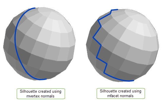
Figure 105-1 Silhouettes generated using mvertex and mfacet normals

For more information on mfacet and mvertex normals, see Section 88.3, “Mesh normals”.

105.3.4 Sharp mfins

This option specifies whether to render sharp mfins on faces with facet geometry. You can use PK_MFIN_is_sharp to find out if a given mfin is sharp. See Section 88.3.2.4, “Finding sharp mfins in meshes” for more information on sharp mfins.

The sharp_mfins option takes the following values:

When sharp_mfins is set to PK_render_sharp_mfins_yes_c, polylines that run along chains of connected sharp mfins will be rendered for every face that contains facet geometry. If the polyline lies along a silhouette, only the sharp mfin polyline is output. If an edge is coincident with a chain of sharp mfins, only the edge is output.

Figure 105-2 shows a single face body with a cube-shaped mesh attached with wire edges on the face. The wire edges on the face are partially coincident with a chain of sharp mfins therefore only the edge is output in the region of partial coincidence. See PK_TOPOL_render_line_o_t for more information on how sharp mfins are rendered.

For a list of the visibility codes that can be output by the GO, see Section 4.4.2.6, “Coincidence with sharp mfins” in the Downward Interfaces.

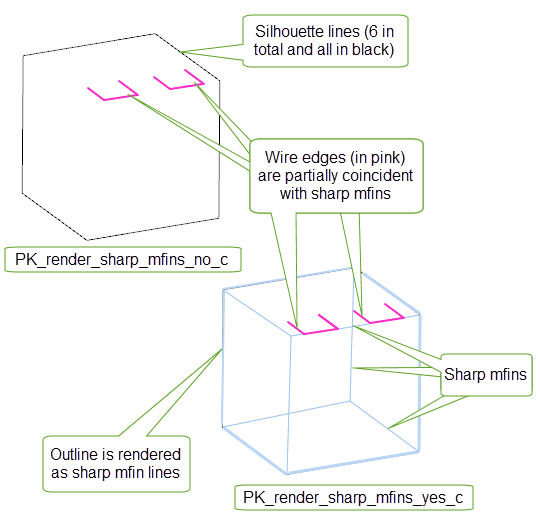
Figure 105-2 Rendering sharp mfins of a mesh cube

105.3.5 Visibility

A hidden-line drawing classifies all lines (edges, silhouettes and hatch lines) according to their visibility, which in turn depends on the view supplied. PK_TOPOL_render_line returns lines and associated visibility codes that represent the type of line returned (e.g., fully visible, hidden by a face, hidden by another edge etc.).

It is your decision as to how to render each type of line from your GO; Parasolid merely returns visibility codes and does not decide how the lines should appear. For example, you can opt to render all hidden lines in the same manner (regardless of what they are hidden by); or you may wish to exclude altogether those lines that are hidden by other lines, to avoid cluttering the diagram. The following table presents the values for the visibility option:

You can find a complete list of all the visibility codes that can be output by the GO in Section 4.4.2, “Line type”, of the Downward Interfaces manual.

Figure 105-3 and Figure 105-4 illustrate the effect of all of the visibility values except for PK_render_vis_extended_c.

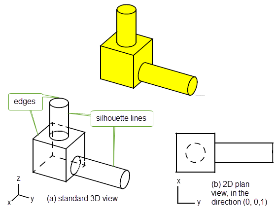
Figure 105-3 A block with bosses, shown from two different directions

Figure 105-3 shows a block with two bosses, as seen from a standard three-dimensional view and also a two-dimensional plan view with view direction (0 0 1) (i.e., from below the object).

Figure 105-4 shows some sample hidden-line drawings based on what would be seen if you were looking at the object from the plan view shown in Figure 105-3(b), although the pictures are actually shown from the standard 3D view.

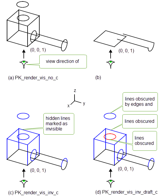
Figure 105-4 Rendering Figure 105-3 with different values of the visibility option

In diagram (a) above, all lines are rendered, as they are all marked as visible. Note that the silhouette lines for the upper boss are not rendered, because in the view direction (0, 0, 1) this boss has no silhouette. In diagram (b), no hidden lines are rendered, as they have not been returned by the function. In diagram (c), all lines are rendered but those that are hidden are displayed differently. The same is true in diagram (d), where an additional distinction between lines hidden by edges or faces is made.

The visibility option PK_render_vis_extended_c enables the invisible , drafting , and self_hidden options: see sections Section 105.3.6, “Invisible”, Section 105.3.7, “Drafting”, and Section 105.3.8, “Self-hidden” respectively. These let you specify more precisely how the GO data should differentiate between different cases of obscured lines. These three options are ignored if visibility is not set to PK_render_vis_extended_c.

When displaying hidden lines (using either PK_render_vis_inv_c, PK_render_vis_inv_draft_c, or PK_render_vis_inv_extended_c), you can prevent the display of hidden lines on specific bodies passed to PK_TOPOL_render_line. See Section 105.3.22, “Suppressing hidden lines in bodies in an assembly” for details.

105.3.6 Invisible

This option specifies whether invisible lines are output when visibility is set to PK_render_vis_extended_c.

The resulting GO output is described in Section 105.3.22, “Suppressing hidden lines in bodies in an assembly” section.

When invisible is PK_render_invisible_yes_c, you can prevent the display of invisible lines on specific bodies passed to PK_TOPOL_render_line. See Section 105.3.22, “Suppressing hidden lines in bodies in an assembly” for details.

105.3.7 Drafting

This option determines whether or not a distinction is made between lines hidden by lines and lines hidden by faces when visibility is set to PK_render_vis_extended_c.

The resulting GO output is described in Section 105.3.22, “Suppressing hidden lines in bodies in an assembly” section.

105.3.8 Self-hidden

This option is used to determine whether a distinction is made between lines hidden by faces of their own occurrence (i.e., from the same connected body) and lines hidden by faces of another occurrence (i.e., from a separate body or component of a disjoint body) when visibility is set to PK_render_vis_extended_c. Lines that are hidden by faces of their own occurrence are called self-hidden.

Figure 105-5 shows the effect of each value of self_hidden , where invisible is PK_render_invisible_yes_c and drafting is PK_render_drafting_yes_c.

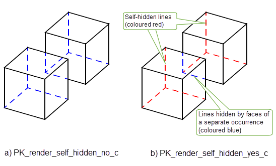
Figure 105-5 The effect of the self_hidden option

105.3.9 Smoothness

The smooth option generates additional graphics output data which specifies whether an edge is “smooth”, “not smooth” or “smooth but coincident with a silhouette” (for view-dependent and hidden-line drawings only).

The value for smooth indicates whether the direction of the normal to the surface varies continuously across the edge or not. Examples of smooth edges are blend boundaries and edges which have been scribed onto a face.

If the option is not given, all edges are output with their smoothness code set “unknown” (CODUNS).

Although an implementation of GO may choose to ignore smooth edges, (those output with smoothness code CODSMO), it must draw ones classified as coincident with a silhouette (marked with code CODSMS) or gaps will occur in the drawing, where the obscured silhouette line was found.

The PK_render_smooth_draft_c setting is a specialized option which detects cases where smooth edges are coincident with lines (other than silhouettes) and reclassifies these before output through GO as being obscured by the faces of the smooth edge (i.e. tagged as CODDRV) rather than being obscured by the smooth edge itself.

The reason for the option is to provide support for implementations of GO which simply ignore smooth edges; it avoids the case where a smooth edge obscures part of another edge and ignoring it would cause gaps in the drawing.

There is no need to use the smoothness option if your GO does not use smoothness data.

105.3.10 Tolerance on smooth edges

You can use the following two options to specify a tolerance within which an edge is considered smooth:

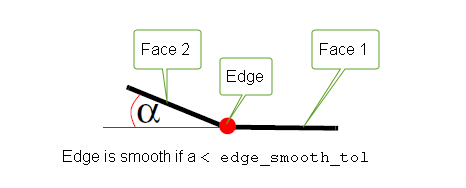
Figure 105-6 Angular tolerance for smooth edges

105.3.11 Output of internal edges

The internal option is used to specify whether to indicate internal edges, i.e. where faces on either side of the edge lie on the same surface.

If the internal option is set to PK_render_internal_no_c, the GO data is output with the internal edge value set to ‘unknown’ (CODINU). If it is set to PK_render_internal_yes_c, Parasolid will calculate and output whether the edges are:

• internal edges (CODINE)
• internal but coincident with a silhouette (CODINS)
• not internal edges (CODNIN)

The application can decide whether to suppress drawing these edges.

105.3.12 Sketching bodies that have missing geometry

You can use the ske_missing option (PK_render_ske_missing_t) in PK_TOPOL_render_line to control whether Parasolid attempts to render bodies that have missing geometry information. Generally, rendering is best performed on bodies whose geometry is completely specified. However, there may be times - for example if you are attempting to work with model data that has been imported from another source - when it is useful to be able to visualise a body that has missing information.

The ske_missing option takes the following values:

105.3.13 Ignoring small features

This option allows small features to be ignored, where a small feature is a set of connected faces whose box is smaller than a user-specified value. The small feature is replaced by a loop of edges which indicates the position of the boundary between the small feature and the model. These loops are either completely visible or invisible (see Figure 105-7).

The options available for ignore are:

If ignore is set to PK_render_ignore_absolute_c then any feature whose size box is smaller than this value is ignored. If ignore is set to PK_render_ignore_ratio_c then the value input corresponds to the ratio of the feature box size to the size of the box containing the model, i.e. if this value is set to 0.01 then a feature is ignored if its box is smaller than 1% of the model’s box.

Not all small features are ignored. This is determined by the position of the boundary between the small feature and the rest of the model, only if this boundary lies completely within a face of the model is the small feature ignored.

In the left-hand illustration of Figure 105-7 the boundaries of the small features lie completely within another face in the model. These features are replaced by a loop of edges indicating where the features lie on the model. Each edge in these loops is still output, but is labelled with the code ‘CODIGN’ where it would normally have its ‘internal’ property output. See PK_GOSGMT_f_t, in the PK Interface Programming Reference Manual for information about CODIGN.

In the right-hand illustration of Figure 105-7 the boundaries of the small features lie across the boundary of two faces. These features cannot be ignored.

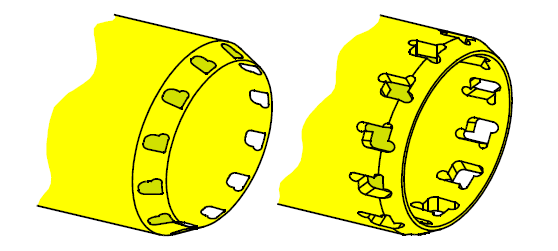
Figure 105-7 Ignoring small features - demonstrating small features that can be ignored and those that cannot.

105.3.14 Hierarchical output

The hierarchical output option can be used when rendering a hidden-line drawing. It specifies that edges/silhouettes/hatch lines must be output through GO hierarchically, consisting of two calls to GOSGMT, enclosed by a pair calls to GOOPSG and GOCLSG.

The first call to GOSGMT defines the line segment type and its geometry.

The second call to GOSGMT defines a “visibility segment” (SGTPVP), specifying points at which the segment visibility or smoothness changes and the visibility codes for edges/silhouettes/hatch line between these points.

If geometry is being output in polyline form, there is an option which outputs an additional parameter with each visibility transition point corresponding to its position along the polyline.

The PK_render_hierarch_no_geom_c option can only be used if the segment geometry has been output in an earlier call to PK_TOPOL_render_line and has been stored by the application.

See Section 4.3.1, “Segment hierarchy” in the Downward Interfaces manual for more information.

105.3.15 B-Curve format

This option specifies which format is used by the graphics output functions to output rendering data for B-curves. This applies to B-curves which are defined in the model and to derived B-curves such as hatch and boundary lines on B-surfaces.

Curves are output in rational or non-rational form; depending on the order of the original curve or surface from which is was derived.

See Appendix B, “The Mathematical Form Of B-Geometry” for further information.

105.3.16 Controlling memory usage

You can let your application have a degree of control over the amount of system resources during hidden-line operations using the memory_target and memory_target_value options for PK_TOPOL_render_line. These options let you specify a peak memory value that Parasolid attempts to keep within during the call to PK_TOPOL_render_line.

Controlling memory usage during hidden-line operations can be useful for:

• Rendering extremely large assemblies that require more memory than the total resource of the host machine.
• Rendering smaller assemblies within the available RAM of the host machine, without resorting to virtual memory.

Although this technique results in an increase in total processor time, in certain cases it can result in a decrease in the elapsed (real) time taken to render the assembly.

Parasolid does not guarantee to meet the specified target.

Using this option can bring varying degrees of success, depending on the target you specify, the resources available on the machine, and the size of the assembly that you are rendering. Different memory targets and different assemblies may yield improvements in memory usage, or elapsed time taken to render, or both.

Your application could typically follow these steps in order to calculate a suitable target memory value:

• Calculate the amount of free RAM available to your application and Parasolid. This might include both physical RAM and virtual RAM, or just the former, depending on whether you wanted to use virtual memory.
• Estimate the amount of memory (or choose a proportion of the available free RAM) that is needed by your application to process graphical output from PK_TOPOL_render_line.
• Subtract these two values to arrive at an optimal target value for Parasolid memory usage.

For large assemblies, a memory target in the region of 100MB may be possible, regardless of the original memory requirement. Using this option may let you render some assemblies successfully that would otherwise be impossible to display.

105.3.17 Reporting line fit failures

You can use the report_lines option to report whether there are any model curves to which Parasolid could not fit polylines during rendering. This takes the following values:

If report_lines is set to any of the above values except PK_render_report_line_no_c, a Parasolid Report of type PK_REPORT_record_type_3_c is generated with a status of PK_REPORT_3_line_fit_tols_c and returns information for curves where the line fit has failed.

See Chapter 11, “Using Reports”, for more information about the Parasolid Report mechanism.

105.3.18 Hatching

Parasolid supports planar hatching, radial hatching and parametric hatching.

Planar hatching can be expensive to calculate for some types of surface, hence the other, surface-specific types of hatching.

When constructing hidden-line drawings, hatch lines are classified as visible/invisible in a similar way as used when drawing the model edges.

105.3.18.1 Planar hatching

Planar hatching instructs the function to output lines representing the intersections of a face with a family of equally spaced parallel planes.

The planar_hatching value defines the hatch spacing in model units.

The axis field of planar_axis specifies the normal direction of hatch planes.

The location field of planar_axis defines a point on one of the hatching planes which allows the application to control the relative position of hatch lines on a face. This option allows the application to simulate more complex hatch spacing by varying the location and calling PK_TOPOL_render_line multiple times.

The PK_render_planar_free_c option specifies that Parasolid should choose the start position for hatching.

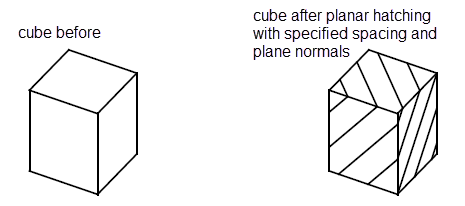
Figure 105-8 Planar hatching (both cubes drawn with PK_TOPOL_render_line)

105.3.18.2 Radial hatching

Radial hatching is used on cylindrical, spherical, conical, toroidal and blending faces (described below as radial faces).

The radial hatching parameters allow cross-hatching of faces to be specified, such as producing lines both along and around a cylinder.

The initialised values of zero imply that hatching is not required in a particular direction (the full meaning depending on the surface types).

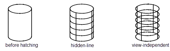
Figure 105-9 Radial hatching using radial_around = pi/2 to control vertical hatch lines and radial_along = 7 to control the spacing between the circular hatch lines

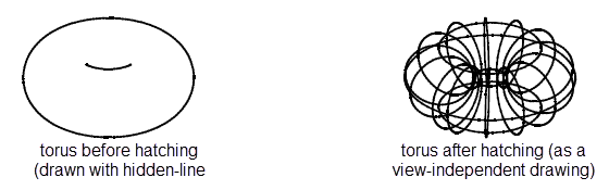
Figure 105-10 Radial hatch (using the same option data as Figure 105-9)

The hatched torus looks messy using this value of radial_along to control the spacing between the circles centered on the spline.

If we use the radial_about value instead, to control this spacing by giving an angle to use between the planes which produce these intersection circles, it is much easier to control what happens.

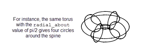
Figure 105-11 Radial hatching using all three data options

Cylindrical and conical surfaces

The interpretation of different radial values for cylindrical and conical surfaces is as follows:

radial_around

radial_along

radial_about

radial_around_start

radial_along_start

radial_about_start

Spherical surfaces

The interpretation of different radial values for spherical surfaces is as follows:

radial_around

radial_along

radial_about

radial_around_start

radial_along_start

radial_about_start

Toroidal surfaces

The interpretation of different radial values for toroidal surfaces is as follows:

radial_around

radial_along

radial_about

radial_around_start

radial_about_start

radial_along_start

Edge-blend surfaces

The interpretation of different radial values for edge-blend surfaces is as follows:

radial_along

radial_around

radial_about

radial_along_start

radial_around_start

radial_about_start

105.3.18.3 Parametric hatching

Parametric hatching instructs the function to output data corresponding to parametric hatch lines.

Parametric hatch lines can be output on any type of surface. The lines output are the locus of points of constant parameter on the equivalent B-surface.

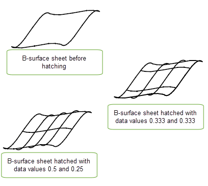
Figure 105-12 Parametric hatching

On faces, the spacing starts at the low parameters of the parameter box of the faces, as returned by PK_FACE_find_uvbox.

105.3.19 Unfixed blends

This option is only available when drawing view-independent topology.

It instructs the rendering function to draw unfixed blends as they would appear when fixed.

If the entities being drawn are bodies or edges, an unfixed edge is not output directly. Instead the edges of the faces adjacent to the edge are clipped and rib lines are added at each end of and possibly along the spine of the unfixed blending edge.

If an unfixed blended edge is drawn in isolation, no other graphical information about the attached faces is output.

The parameters of an unfixed blend are held as a blended attributes. These describe the start and end radii and possibly a specific rib spacing distance to use when the unfixed blend is drawn.

105.3.19.1 Options

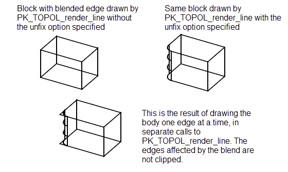
Figure 105-13 Unfixed blends, drawn with and without surrounding edges

105.3.20 Overlapping bodies

Parasolid allows assemblies and lists of bodies that overlap in model space to be rendered with hidden lines such that the results are predictable and stable. Where the edges and silhouettes of one body intersect with the face of another, those lines are trimmed to the intersecting face. New intersection curves can also be generated, although this does incur a performance overhead. In these cases, however, the overhead can be minimised if you know which bodies are likely to overlap.

The values available for the overlap field are:

Figure 105-14 demonstrates the effect of each of these settings on a rendered image. It shows a cylinder passing through a cylindrical hole drilled in a block; the diameter of the cylinder being slightly larger than the diameter of the hole so that the cylinder and the block overlap.

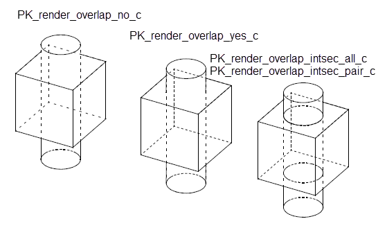
Figure 105-14 Overlapping bodies: demonstrating the effect of the overlap option on a rendered image

In Figure 105-14, when overlap is set to PK_render_overlap_no_c, Parasolid does not detect that the silhouettes of the cylinder intersect the block and they are not output with the correct visibility.

When overlap is set to PK_render_overlap_yes_c, the silhouettes of the cylinder are intersected with the face and rendered correctly.

When overlap is set to PK_render_overlap_intsec_all_c or PK_render_overlap_intsec_pair_c, the silhouettes of the cylinder are intersected with the face and rendered correctly, with new edges generated where the faces of the overlapping bodies intersect.

When generating new intersection curves and edges, if you know which bodies are likely to overlap, you can optimise the performance of Parasolid by using the overlap_indices1 and overlap_indices2 arrays. These arrays take indices of specific bodies in the topols array (as passed to PK_TOPOL_render_line), enabling you to restrict the checks performed by overlap to just these bodies. The following table describes the combinations available, depending on the value of overlap :

105.3.21 Transparency

Bodies can be rendered so that they appear transparent, such that they do not hide other bodies, as shown in Figure 105-15.

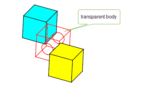
Figure 105-15 A transparent cube with cylindrical hole between two solid cubes

If a body is rendered as transparent it will not hide its own lines, and will not hide the lines of other bodies, as shown in Figure 105-16.

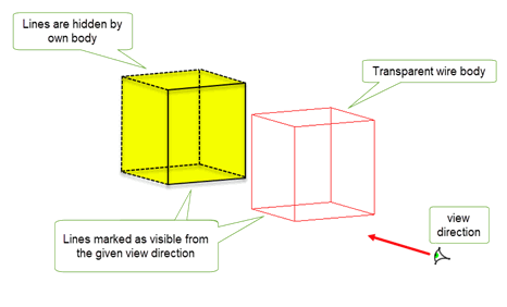
Figure 105-16 Hidden lines when rendering a wire body as transparent, viewed in front of a solid body

There are two ways that a body can be rendered transparent:

• Attach a system attribute of type SDL/TYSA_TRANSPARENCY to the body.
• Add the integer value corresponding to the position in the topols array of an occurrence of the body to the transparent_indices array in PK_TOPOL_render_line_o_t.

You can choose which of the above methods is used using the transparency option in PK_TOPOL_render_line_o_t, which takes the following values:

The transparent_indices array contains the index values of body occurrences that you want to render transparent, according to the position of those occurrences in the topols array. For instance, if you want to render transparent the body occurrences that are in the first, third, and fourth positions of the topols array, transparent_indices should be (0, 2, 3). In this case, n_transparent_indices is 3.

You can also use the transparent_hid option to control how transparent entities are rendered. By default, transparent entities are rendered as transparent, as shown in Figure 105-15. However, if transparent_hid is set to PK_render_transp_hid_yes_c, transparent entities are rendered as opaque relative to themselves and other transparent bodies, but transparent relative to non-transparent bodies. Figure 105-17 demonstrates this setting: the transparent body is drawn as opaque relative to itself (you cannot see its own hidden lines), but transparent with respect to the non-transparent body behind it.

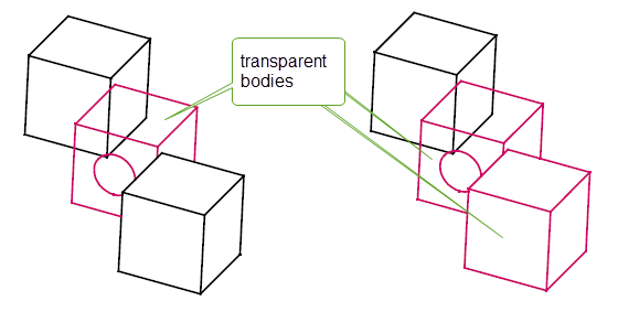
Figure 105-17 Rendering transparent bodies as opaque

105.3.22 Suppressing hidden lines in bodies in an assembly

If you are rendering a hidden-line view containing several bodies, you can switch off hidden-line display for specific bodies. This can have benefits in terms of:

• Performance - by switching off hidden lines in parts of an assembly that are of less interest to the user, you can improve the performance for rendering the whole assembly.
• Clarity - by omitting hidden lines from specific bodies, other details can be more readily viewed (see Figure 105-18).

You can prevent hidden lines in specific bodies using the suppressed_indices option. This is a list of indices into the topols passed to PK_TOPOL_render_line that indicates which bodies should have no hidden lines.

For example, if three bodies are passed as topols , and you want to suppress hidden lines in the first and third of these, set suppressed_indices to [0 2] , and the accompanying n_suppressed_indices option to 2 .

Figure 105-18 shows an example in which a total of six bodies are rendered using the view direction shown.

• Figure 105-18 (a) shows the configuration of these bodies and the view direction used.
• Figure 105-18 (b) shows the effect when hidden lines are displayed in all the bodies. Because the hidden back face of the front body is corrugated, it is difficult to see details of the bodies behind it due to the hidden lines generated for the corrugated face.
• Figure 105-18 (c) shows the effect when suppressing hidden lines in the front body. When you do this, there are no hidden lines generated for the corrugated face, and details for the other hidden bodies are clear.

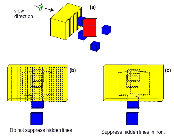
Figure 105-18 Suppressing hidden-line display in specific bodies in an assembly

105.3.23 Using viewports to render specific entities

Parasolid lets you specify one or more viewports - discrete volumes of three-dimensional space - so that you can control which entities in a body are rendered. This is a particularly useful way of improving rendering performance in cases where you are performing modelling operations on a large body that only change a small number of entities, or entities in a discrete part of the body: by specifying a viewport, only the entities that are inside that viewport are re-rendered.

Parasolid lets you specify:

• How many viewports to use.
• What type of viewports to use.
• Whether or not to clip the rendered portions to the boundary of the viewport itself.

This section describes how to use viewports to render large bodies efficiently.

105.3.23.1 Using single or multiple viewports

Generally when you use viewport functionality, you only want to specify a single viewport. Sometimes, however, it might be useful to use several viewports in a single call to PK_TOPOL_render_line; if, for instance, you want to re-render discrete changes in different components of a disjoint body.

You use the viewport option in PK_TOPOL_render_line_o_t to specify whether to use single or multiple viewports. This takes the following values:

A single viewport is specified using the viewport_sf option. This takes a standard form for a single non-aligned box.

When multiple viewports are used, viewport_sf is ignored, and the viewports are specified using the following options:

n_viewports

viewports

105.3.23.2 Types of viewport

Whether you use a single viewport or multiple viewports, Parasolid supports two different kinds of viewport: 3D and 2D viewports. Both of these are defined using a non-aligned box (PK_NABOX_sf_t).

You use the viewport_type option to specify the type of viewport. The default type of viewport is 3D (PK_render_viewport_type_3D_c).

Figure 105-19 illustrates the differences between typical 3D and 2D viewports onto a body; these viewports could be specified using the same non-aligned box.

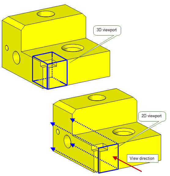
Figure 105-19 Specifying 2D and 3D viewports on a body

105.3.23.3 Clipping entities to viewport boundaries

Usually, some entities in a body cross the boundary of a viewport; they are not entirely contained within the definition of the viewport itself. Parasolid provides the viewport_clipping option to let you control whether such entities are completely rendered, or whether the rendering is clipped to the boundary of the viewport itself. The viewport_clipping option takes the following values:

Using the same viewports and body illustrated in Figure 105-19, Figure 105-20 shows the entities that are returned for a 3D viewport when clipping is on or off (clip lines are shown in green), and Figure 105-21 shows the entities returned for a 2D viewport when clipping is on or off.

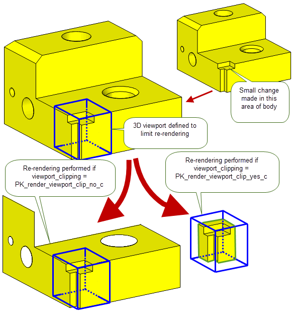
Figure 105-20 Clipping a 3D viewport

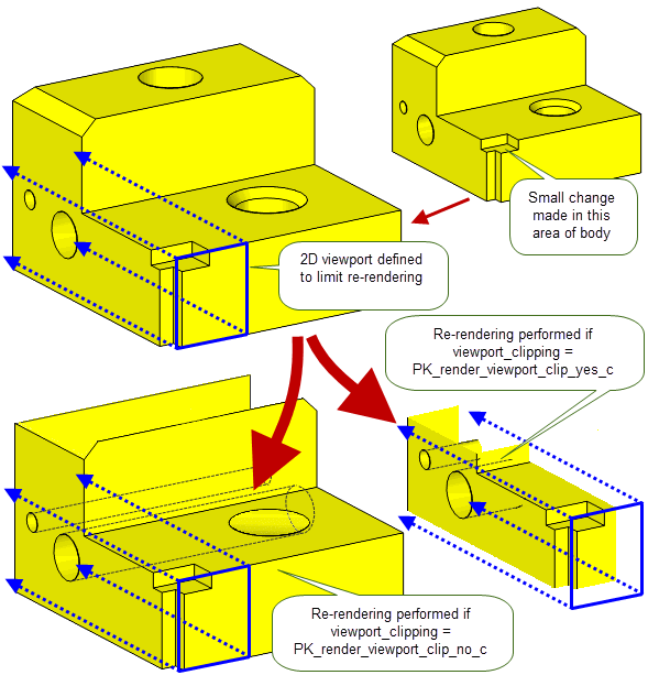
Figure 105-21 Clipping a 2D viewport

105.3.24 Regional data

The region option can be used when rendering a hidden-line drawing. It generates additional graphics output data which allows your application to analyse the projected (2-dimensional) hidden-line picture into distinct regions and link up the boundaries of the regions appropriately.

There is no need to use this option if your GO does not use such regional data. The region option takes the following values:

Regional data is attached to all boundary line segments, that is, to edge, silhouette, interference, and clip segments, and is output as follows:

• If PK_render_region_yes_c is used, all visible lines have regional data.
• If PK_render_region_attrib_c is used, all lines bounding visible portions of faces that have the regional attribute are output with regional data. In this context, bounding means (an edge) adjacent to, or (a silhouette) lying on, the face, or (an edge or a silhouette) coming between the face and the eye and dividing a visible from an invisible part of the face.

When the hidden-line picture is projected into two dimensions, the lines divide the plane into distinct regions, as shown in Figure 105-22.

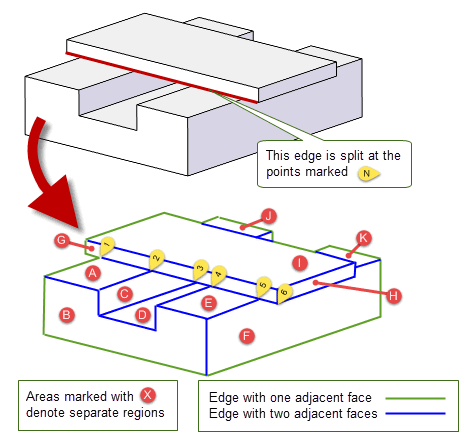
Figure 105-22 Regional data - hidden-line picture

For each region that derives from a face, the lines whose projections in the plane bound the region are all output with regional data. This data indicates which points in the image bound the line, and which faces are on each side of the line. Your application can then construct the loops and regions of the image. If region is PK_render_region_attrib_c, then regional data is only output for lines bounding regions that derive from faces that have a SDL/TYSA_REGION attribute attached.

For information about how regional data is output, see Section 4.5, “Interpreting regional data”, in the Downward Interfaces manual.

[back to top]