| |
Graphical Output |
| <<< File Header Structure | Chapters | Registering the Frustrum >>> |
When a call is made to the PK rendering functions, the graphical data generated is output through a set of functions known as the GO (Graphical Output) Interface
|
Note: You should not call heavyweight functions from the GO. See Section 120.2.1, “State of the code in execution”, of the Parasolid Functional Description for more information on heavyweight functions. See the Function Exclusivity list in the PK Interface Programming Reference Manual to find out if a function is heavyweight or lightweight. |
Line Data is produced by PK_GEOM_render, PK_TOPOL_render_line and PK_TOPOL_render_facet. It is output through the GO functions GOOPSG, GOSGMT and GOCLSG.
There are two values which GO functions should return in the ifail argument, both defined as tokens in the Parasolid failure codes include file. All GO functions should return one of:
Data output through the GO is organised into segments, which correspond to identifiable portions of the model (not necessarily entities in the Kernel sense).
There are two classes of segment:
Every segment has a type, which governs (among other things) whether it is a hierarchical segment or not.
Single level segments always contain the data for a line to be drawn, as well as information about what kind of line it is.
Hierarchical segments usually contain other segments. Note that graphical data is always output hierarchically: using the
hierarch
option in PK_TOPOL_render_line affects the level of hierarchy.
hierarch
option is used then edge segment SGTPED; silhouette segment SGTPSI; and hatch-lines SGTPPH (planar) SGTPRH (radial) SGTPPL (parametric) are hierarchical.For example, after a request by the application for view-dependent topology information by a call to PK_TOPOL_render_line, a hierarchical segment is opened for each body. Data for each silhouette line is then given in a single-level segment, and each is contained wholly within the hierarchical segment of the corresponding body.
A single body segment is not guaranteed to contain data for the whole body - for example, sometimes the kernel can output part of a body, close the body segment, open and close another body segment, and then open a new segment for the first body, and output the rest of it.
Assemblies constructed with KI routines must be flattened and their constituent body tags and transformation matrices copied into entity arrays before they can be rendered by the PK functions. For further information see Chapter 1, “Parasolid KI Programming Concepts”, of the Parasolid KI Programming Reference Manual.
All such body segments have a unique occurrence number when they are rendered - this number is the index of the body (in the entity array) plus 1.
The tags associated with each of these body segments are likely to be different. There are two circumstances when you could receive separate body segments with the same tag:
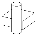
Figure 4-1 Hidden line drawing of a single body
In this case, the lines comprising each visible portion of the body might be output in separate body segments.
You should note that geometrical data output through the segment output functions is:
The application must transform all of the received GO data by a viewing matrix before projecting the data into two dimensions:
view_transf
argument when calling PK_TOPOL_render_lineIf the viewing matrix specifies a parallel orthographic projection, the 3D GO data can be projected into 2D form simply by replacing the third column of the matrix by a zero vector:
See Appendix B, “Graphical Output Functions”, for detailed descriptions of each function. The three functions (GOOPSG, GOSGMT, GOCLSG) all have the same arguments, but interpret them in different ways. The arguments are:
GO....( segtyp, ntags, tags, ngeom, geom, nlntp, lntp, ifail )
The first argument of each function is an integer
segtyp
. Parasolid always sets this to the token representing the
segment type. These tokens are listed in Appendix I, “Go Tokens and Error Codes”, of this manual. The different types of segment are discussed in a later section.
The values of some of the arguments to the segment functions, and therefore how you should interpret them, vary depending on the segment type. The arguments to which this applies are noted as such, below. The remaining arguments are pairs of integers and arrays.
The integer
ntags
gives the length of the
tags
array. The contents of this array depend on the segment type. For example, for a hierarchical body segment,
tags
contains the tag of the body; for a single level edge segment,
tags
contains the tag of the edge.
The integer
nlntp
gives the length of the
lntp
array. This is an array of integers, the first of which is always the
occurrence number of the segment, and the rest of which are tokens. For hierarchical segments (i.e. in calls to GOOPSG and GOCLSG) the
lntp
array contains only the occurrence number of the segment.
Occurrence numbers link the segment to the entity which was passed to the rendering function. You can use them to associate the segments with the Parasolid entities (perhaps using identifiers to identify them). You can then identify what a particular line represents, and the entity it belongs to.
See also Section 103.3.2, “Occurrence numbers” in the Parasolid Functional Description.
Silhouettes are produced by the
silhouette
option in PK_TOPOL_render_line. These automatically have each silhouette on a face labelled with a different integer, i.e. 1, 2, 3, etc.
The remaining array entries, which are given as well as the occurrence number for all single-level segment types, are as follows.
Line type specifies the type of geometry of the curve or lattice element which the segment represents. This is one of:
The different types of line are discussed in detail under Section 4.4.3, “Geometry”, below. They are defined by tokens of the form “L3TP...”
Completeness codes indicate whether a segment represents a complete item or is part of a larger item. The codes returned may be any of the following:
For more information about viewports, see Section 104.3.23, “Using viewports to render specific entities” in the Parasolid Functional Description.
Completeness codes are only calculated in a hidden line drawing, so segments output from a view independent or view dependent wireframe drawing has code CODUNC (unknown completeness).
Visibility specifies that the line is visible, invisible or of unknown visibility. This value is only relevant to hidden line pictures, so all segments produced in view independent or view dependent wireframe drawings have unknown visibility (CODUNV).
visibility
field of the PK_TOPOL_render_line option structure.The effects of the PK_render_vis_... options are as follows:
|
no visibility evaluated (topology is output as a view-dependent wireframe drawing) |
|
|
lines are output subject to the ‘invisible’, ‘drafting’ and ‘self-hidden’ fields of the PK_TOPOL_render_line option structure |
Smoothness indicates whether a line is smooth (i.e. the normals of the faces either side of the edge vary smoothly across it). Blend boundaries are smooth by definition. This code is provided because sometimes you may wish to leave smooth edges out of your pictures, to make them look more realistic.
For further information see Section 104.3.24, “Regional data” in the Parasolid Functional Description.
CODSMS is a special code which can be returned only from a hidden line drawing. It indicates that an edge is smooth, but that it is also coincident with a silhouette line which is not output. In this case you need to draw the edge even though it is smooth, because otherwise the silhouette is missing, making the picture look wrong.
CODNSS is a special code which can be returned only from a hidden line drawing when rendering sharp mfins. It indicates that the mfin line (which is sharp) is coincident with a silhouette line which is not output.
If regional data was requested from a hidden line drawing, edge and silhouette segments are output with start and end point indices. These are output only when the regional data option is specified, and allow the line segment to be linked correctly with other lines. See Section 4.5, “Interpreting regional data”, for more information.
If sharp mfins were requested then edge segments are output with a code describing whether the segment lies on a chain of connected sharp mfins as follows:
These codes are only output for edge segments when the
sharp_mfins
option in PK_TOPOL_render_line is set to PK_render_sharp_mfin_yes.
See Section 4.4.4.19, “Sharp mfin line: SGTPSF” for more information.
For hierarchical body segments the
geom
array always contains the model space box of the body, and
ngeom
is 6. See Section 4.4.4, “Segment types” for more details.
For a single level segment the
geom
array is an array of real numbers specifying the geometry of the line it represents. The length and contents of this array depend on the line type, as specified by the second entry of
lntp
(see Section 4.4.2, “Line type”). The length of the array is
ngeom
unless otherwise stated. This concept of a
line does not correspond exactly to any type of entity at the PK Interface: it is either a set of data describing an analytic curve with a start-point and an end-point, or a poly-line.
The types of line which can be returned are:
The explicit direction is generally more accurate than that obtained from the start and end points.
Note that the double type array holding a poly-line is of length 3*ngeom.
The poly-line is a chordal approximation to a line which can not be held explicitly within the Kernel. It defines a series of points, each of which lies on the corresponding Parasolid curve. If you join the points of a poly line with straight line segments, this produces an approximation to the curve which is adequate for most viewing purposes. Splining the points produces a more accurate approximation if one is required.
L3TPFV and facet strip vertices - L3TPTS
L3TPFN; and facet strip vertices plus surface normals - L3TPTN
L3TPFP; and facet strip vertices plus parameters - L3TPTP
L3TPFI; and facet strip vertices plus normal plus parameters - L3TPTI
The number of b-spline vertices is supplied in the 9th element of the integer array and the number of knots is supplied in the 10th element of the integer array.
The number of b-spline vertices is supplied in the 9th element of the integer array and the number of knots is supplied in the 10th element of the integer array.
L3TPF1; and facet strip vertices + normals + parameters + 1st derivatives - L3TPT1
L3TPF2; and facet strip vertices + normals + parameters + all derivatives - L3TPT2
As stated earlier, the first argument of each segment output function is the segment type. A segment of a particular type is always of the same class:
hierarch
option is used (like bodies, they cannot be output by GOSGMT, only by GOOPSG and GOCLSG)
hierarch
option isn’t used they are all
single-level (and therefore are only output by GOSGMT)The segment types with their dependent data are as follows.
This type of hierarchical segment corresponds to an occurrence of a body in the model. If an entity within a body is passed to a rendering function, Parasolid still opens the body segment with GOOPSG before outputting the requested entity, and closes the body segment afterwards. This lets you build a graphical data structure and subsequently update it.
tags
holds the tag of the body
ngeom
is 6 and
geom
holds the model space box of the body, in the order: xmin, ymin, zmin, xmax, ymax, zmax. There is no geometric data apart from the body box, as all the lines which make up the body in the picture form separate segments within the body segment.
This type of hierarchical segment corresponds to an occurrence of a face in a model. GOOPSG allows you to build a graphical data structure in the same way as for bodies as explained above.
tags
holds the tag of the face
ngeom
is 6 and
geom
holds the model space box of the face, defined in the same way as the body box, as described above.The following are all single-level segment types which may be output by GOSGMT:
These represent edges or portions of edges. They are produced by PK_TOPOL_render_line if you specified the
edge
option. An edge segment may be a complete edge (E) of the model or may be only part of an edge, for example:
invisible
or
drafting
options are used, the invisible portions of (E) are also output by further calls to GOSGMT.
tags
contains the tag of the edge in the model.
tags
contains the tag of the edge in the model and two extra tags, identifying the faces either side of the line in the 2-dimensional drawing. Either or both of these face-tags may be PK_ENTITY_null.
If regional data is required
lntp
contains two extra integer values: the indices of the start and end points of the line (see Section 4.5).
A silhouette is a line on a single face curving away from the eye where its surface changes from visible to hidden. Both view dependent topology and hidden line drawings produce silhouettes. They may be output whole, or cut or shortened in the same way as for edges, see above.
tags
contains the tag of face bearing the silhouette.
tags
contains two extra tags, and
lntp
contains point indices, as for edges.See Section 4.5, “Interpreting regional data”, for information on regional data.
This is a further way of rendering an unfixed blend: adding lines across the blend surface, roughly perpendicular to the original edge. Rib lines can be drawn as well as a blend boundary, but not instead of it. As for blend boundaries, rib lines can only be produced by a view independent drawing.
If an edge with an unfixed blend is being rendered as view independent topology with unfixed blends, the blend is rendered instead of the edge. The way in which the blend is rendered depends on the option data provided with the unfixed blend option, or if this is absent, on the attribute data associated with the blend. Unfixed blends are ignored by all the other rendering functions.
See the Section 104.3.19, “Unfixed blends”, in the Parasolid Functional Description manual for further information on rendering unfixed blends.
A blend boundary is the line where the blending surface meets the faces or other blends adjacent to the edge.
tags
contains the tag of the face.
A facet is a planar or near planar polygon. A face rendered by the facet rendering function is approximated by a collection of contiguous facets. The data supplied is dependent on the setting of the rendering options to the faceting function.
See Chapter 106, “Facet Mesh Generation” and Chapter 107, “Faceting Output Via GO” in the Parasolid Functional Description manual for further information on faceting.
tags
contains the tag of the face on which the facet lies.
tags
contains the tag of the face on which the facet lies and also contains tags of the model edges from which each facet edge is derived. The number of edge tags equals the number of vertices which define the facet. The null tag is supplied if the facet edge is not derived from a model edge. The first edge tag (tag[1]) is the tag of the model edge from which the first facet edge is derived. The first facet edge ends at the first vertex given in the geom array, see below. The second edge tag is for the facet edge which ends at the second vertex in geom, and so on.
lntp
for this segment type:
lntp[2]
contains the number of loops in the facet
lntp[3]
contains the number of vertices in the first loop
lntp[4]
contains the number of vertices in the second loop
ngeom
and
geom
depend on the geometry type of this segment as specified in the second element of
lntp
.If a facet has multiple loops, the outer loop is output first and the inner loops follow. The vertices of the outer loop are ordered counter-clockwise when viewed down the surface normal. The vertices of inner loops are ordered clockwise. Facets are manifold. That is, no vertex coincides with any other in the same facet, nor does it lie in any edge in the same facet.
This type of facet is only produced by the facet drawing function.
When rendering a list of entities, Parasolid may encounter a body, face or edge which it is unable to render (e.g. a rubber face). In such a case, Parasolid outputs an error segment giving the tag of the bad entity a code indicating why it was not rendered. When the error segment has been output, Parasolid continues to render the remaining entities.
Geometric segment types SGTPGC (curves), SGTPGS (surfaces), and SGTPGB (surface boundaries) are used to sketch unchecked parametric curves and surfaces as view independent drawings enabling the relevant curve/surface to be visualised.
If during a call to the facet drawing function, user tolerances can't be matched, or facets are created which self intersect or are severely creased, then geometric data is output as a segment type SGTPMF. In this case, the facets are always triangular.
If PK_TOPOL_render_line is used to output data hierarchically from a hidden line drawing (that is, if the
hierarch
option is anything but PK_render_hierarch_no_c), then the single level segments output for each edge, silhouette, or hatch-line are:
hierarch
is PK_render_hierarch_yes_c or PK_render_hierarch_param_c)
If regional data has been requested,
tags
holds the regional information for the segments between the visibility transition points. This means that
ntags
is twice the value of
nlntp
, since
nlntp
represents the number of visibility code
pairs (see below).
tags[0]
is the tag of the face to the left of the segment after the first transition point
tags[1]
is the tag of the face to the right of the segment after the first transition point
tags[2]
is the tag of the face to the left of the segment after the second transition point
tags[2n-2]
is the tag of the face to the left of the segment after the nth transition point
tags[2n-1]
is the tag of the face to the right of the segment after the nth transition point
If regional data is not requested, then
ntags
is zero and
tags
contains no regional information.For more information on regional data, see Section 4.5, “Interpreting regional data”.
geom
holds the visibility transition points, i.e. the vectors in model space where the edge changes visibility or smoothness.
ngeom
holds the number of these visibility transition points.
The
lntp
array is structured as shown in Figure 4-2 and Figure 4-3. The array consists of five blocks of data, as follows:
nlntp
, holds the visibility codes for the edge.
nlntp
, holds the smoothness codes for the edge. The smoothness property can change along edges which are partially coincident with silhouettes. The smoothness code contained in the geometry segment should be ignored. See Section 4.4.2.4, “Smoothness” for more information.
ngeom
, holds the point indices for the visibility transition points if regional data has been requested.
viewport_clipping
option in PK_TOPOL_render_line_o_t is set to PK_render_viewport_clip_yes_c, then the fourth block, of length
nlntp
, holds the viewport codes describing whether an edge is inside, outside, or coincident with a viewport.
sharp_mfins
option in PK_TOPOL_render_line is set to PK_render_sharp_mfin_yes_c and this visibility segment is for an edge line, then the fifth block, of length
nlntp
, holds the codes describing whether or not an edge lies on a chain of sharp mfins. The sharp mfins code can change along edges which are partially coincident with sharp mfins. Therefore, the sharp mfins code contained in the geometry segment should be ignored. See Section 4.4.2.6, “Coincidence with sharp mfins” for more information.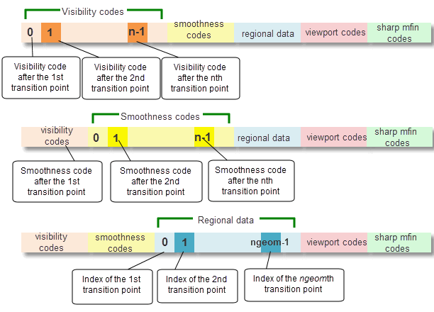
Figure 4-2 Structure of the
lntp
array explaining visibility codes, smoothness codes and regional data
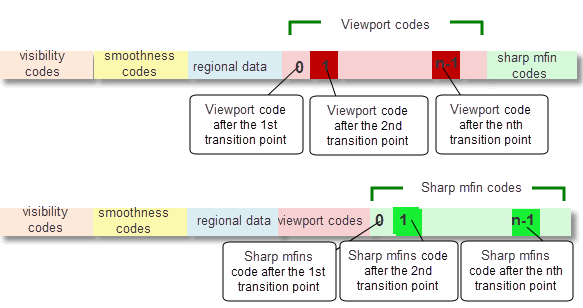
Figure 4-3 Structure of the
lntp
array explaining viewport codes and sharp mfin codes
Using the ‘facet strip’ option when outputting data from the facet drawing function results in this data being output in the form of a ‘strip’ or ‘ribbon’ consisting of triangular facets.
The number of facets in each strip must be specified in the option data list when using this option.
Triangular facets share vertices between adjacent facets with the geometry specifying the vertices of the triangles in a particular order. For example, in a strip consisting of eight triangular facets the order of the vertices are specified as follows:
Figure 4-4 The ordering of vertices in a facet strip
As can be seen from the above example, triangular strip geometry only stores ‘n + 2’ vertices, whereas an individual-triangle’s geometry stores ‘3n’ vertices.
If the
hierarch
option is used to output data hierarchically from a hidden line drawing then the single level segments output for each edge, silhouette, or hatch line is very similar to those output when the other hierarchical options are specified, i.e.
However, when the geometry segment is a polyline, the visibility segment supplied is of type SGTPVP rather than SGTPVT:
ntags
and
tags
are zero, as this information is provided by the hierarchical segment.
ngeom
holds the number of visibility transition points.
geom
holds the visibility transition points. These points are sets of four values, defining both the vector position of the change in visibility and its parameter along the polyline, i.e.
nlntp
holds the number of visibility codes.
lntp
holds the visibility codes for the edge.The parameterisation of polylines is pseudo arc-length, normalized so that the parameter interval of any polyline is always [0,1]. That is, the parameter of any point on the polyline is equal to the distance between the point and the start measured along the polyline, divided by the total length of the polyline.
The parameters are supplied in order to help the application locate the chord in the polyline on which the associated visibility transition point lies.
Given a polyline P with N chords, defined by the set of 3-D points:
we define the total length of a polyline consisting of N chords as:
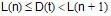
and define distance
D(t) as the length of the polyline at parameter value
t measured from the point  .
.
Given a visibility transition point
v with parameter value  we can find the chord
  on which the point
v lies by finding a point index
n such that
on which the point
v lies by finding a point index
n such that

If, in PK_TOPOL_render_line, overlapping bodies are detected during the rendering process by setting the
overlap
option to PK_render_overlap_intersect_c, then this segment type is used for any curves that are generated as a result of intersections between overlapping faces in the bodies. See Section 104.3.20, “Overlapping bodies”, in the Parasolid Functional Description, for more information.
If, in PK_TOPOL_render_line, 3D viewports are enabled by setting
viewport_type
to PK_render_viewport_type_3D_c and viewport clipping is enabled by setting
viewport_clipping
to PK_render_viewport_clip_yes_c, then any clashes between rendering faces and viewport faces will result in the generation of a clip line. Segments on clip lines are marked with the code SGTPCL. See Section 104.3.23.3, “Clipping entities to viewport boundaries”, in the Functional Description, for more information about viewports.
If, in PK_TOPOL_render_line, sharp mfins are requested by setting
sharp_mfins
to PK_render_sharp_mfins_yes_c then polylines that run along chains of connected sharp mfins will be rendered for every face that contains facet geometry. See Section 104.3.4, “Sharp mfins”, in the Functional Description, for more information.
Lattice segment types SGTPLB (lattice balls), and SGTPLR (lattice rods) are used to render lattice balls as spheres and lattice rods as straight lines between the 2 balls it connects. See Section 104.2.4, “Lattice”, in the Functional Description for more information.
Regional data is produced in a hidden line drawing when you use the
region
option in PK_TOPOL_render_line_o_t. It tells you how to split a hidden line picture into separate 2D regions, as shown in the Figure 4-5.
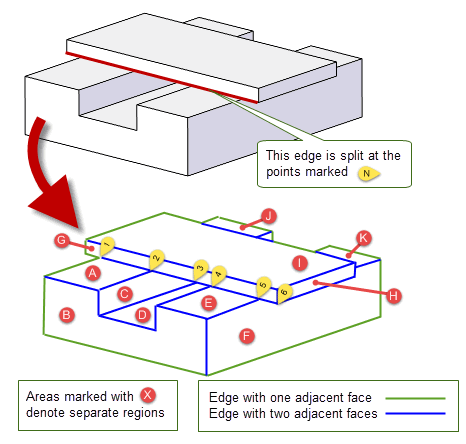
Figure 4-5 Interpreting regional data
A single edge may bound several regions on the two-dimensional picture (for instance the edge marked in Figure 4-5, bounds regions A, C, D, E, F and G). When this happens it is divided at the intersections, and output as several segments, with the same basic segment data (and completeness code CODINC), but different regional data. The additional data is of two types: adjacent faces, and point indices.
The order of faces returned in regional data is based on the orientation of the faces either side of the boundary line in question, relative to the direction of the curve and viewing direction.
When a bounding line is output with regional data, the
tags
array is of length 3 (i.e.
ntags
=3):
tags[0]
contains the tag of the original model entity: either an edge (if the bounding line is generated from a model edge) or a face (if the bounding line is generated from another source, such as a silhouette)
tags[1]
and
tags[2]
contain either the tags of faces in the model, or PK_ENTITY_null. These indicate which faces are on each side of the line corresponding to the segment in the 2D picture. (The faces may or may not be adjacent to the original edge or silhouette in the 3D model.)PK_ENTITY_null indicates that the region of the picture on that side of the line is either part of a face not tagged for regional data or outside the 2D representation of the model (the “outside” of the picture).
Face tags are returned relative to the direction of the line, which is required to interpret the point indices correctly:
tags[1]
is the
left face, and
tags[2]
the
right.
Figure 4-6 illustrates how regional data is returned when rendering three cubes, with a view direction such that only one face from each cube is visible, two of which are partially obscured. The illustration shows how regional data is returned for a sample of edges in the rendered image, shown in red. For simplicity, PK_ENTITY_null is shown as 0 in the illustration, and
tags[0]
is not shown.
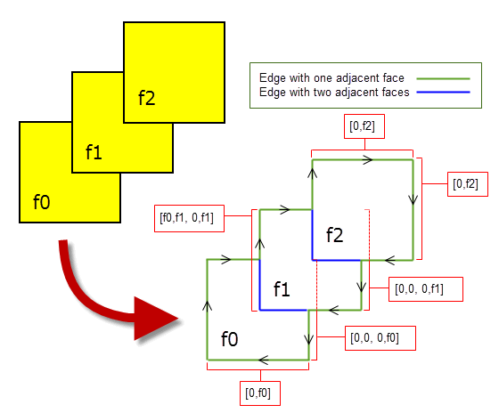
Figure 4-6 Format of regional data for edges
The
lntp
array is of length 7 for a segment with regional data. Elements
lntp[5]
and
lntp[6]
are the
start index and
end index respectively for the line. They are non-zero integer values, and specify which “points” of the two-dimensional picture the segment joins.
Suppose segment A has end index x, and segment B has start index x. Then the end point of A and the start point of B should be regarded as the same point in the two-dimensional picture, even if their geometric projections do not exactly coincide. (This may happen as the result of numerical approximations in rendering.) You will also find that of all the lines sharing a point index, one with it as an end index and one with it as a start index share an adjacent face on the left, and so these two can be linked up as consecutive portions of the boundary of a region; and similarly with faces on the right. The values used for point indices are not in any meaningful order.
Another part of the GO consists of three functions for producing pixel data. These were required to support the KI function RRPIXL. These functions do not need to be implemented to support the PK (they can be supplied in dummy form).
See Appendix J, “Legacy Functions”, for further information on the interface to these functions.
| <<< File Header Structure | Chapters | Registering the Frustrum >>> |
 ( where 0
  )
)